Josephson effect

 The Josephson effect is the phenomenon of supercurrent, a current that flows continuously without any voltage applied, across a device known as a Josephson junction (JJ), which consists of two or more superconductors coupled by a weak link. The weak link can consist of a thin insulating barrier (known as a superconductor–insulator–superconductor junction, or S-I-S), a short section of non-superconducting metal (S-N-S), or a physical constriction that weakens the superconductivity at the point of contact (S-s-S).

Josephson junction array chip developed by the National Institute of Standards and Technology as a standard volt

The Josephson effect is an example of a macroscopic quantum phenomenon. It is named after the British physicist Brian David Josephson, who predicted in 1962 the mathematical relationships for the current and voltage across the weak link.^[1][2] The DC Josephson effect had been seen in experiments prior to 1962,^[3] but had been attributed to "super-shorts" or breaches in the insulating barrier leading to the direct conduction of electrons between the superconductors. The first paper to claim the discovery of Josephson's effect, and to make the requisite experimental checks, was that of Philip Anderson and John Rowell.^[4] These authors were awarded patents on the effects that were never enforced, but never challenged.

Before Josephson's prediction, it was only known that normal (i.e. non-superconducting) electrons can flow through an insulating barrier, by means of quantum tunneling. Josephson was the first to predict the tunneling of superconducting Cooper pairs. For this work, Josephson received the Nobel Prize in Physics in 1973.^[5] Josephson junctions have important applications in quantum-mechanical circuits, such as SQUIDs, superconducting qubits, and RSFQ digital electronics. The NIST standard for one volt is achieved by an array of 20,208 Josephson junctions in series.^[6]

ApplicationsEdit

The electrical symbol for a Josephson junction

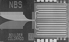
Types of Josephson junction include the φ Josephson junction (of which π Josephson junction is a special example), long Josephson junction, and superconducting tunnel junction. A "Dayem bridge" is a thin-film variant of the Josephson junction in which the weak link consists of a superconducting wire with dimensions on the scale of a few micrometres or less.^[7][8] The Josephson junction count of a device is used as a benchmark for its complexity. The Josephson effect has found wide usage, for example in the following areas.

SQUIDs, or superconducting quantum interference devices, are very sensitive magnetometers that operate via the Josephson effect. They are widely used in science and engineering.

In precision metrology, the Josephson effect provides an exactly reproducible conversion between frequency and voltage. Since the frequency is already defined precisely and practically by the caesium standard, the Josephson effect is used, for most practical purposes, to give the standard representation of a volt, the Josephson voltage standard.

Single-electron transistors are often constructed of superconducting materials, allowing use to be made of the Josephson effect to achieve novel effects. The resulting device is called a "superconducting single-electron transistor".^[9]

The Josephson effect is also used for the most precise measurements of elementary charge in terms of the Josephson constant and von Klitzing constant which is related to the quantum Hall effect.

RSFQ digital electronics is based on shunted Josephson junctions. In this case, the junction switching event is associated to the emission of one magnetic flux quantum ${\displaystyle \scriptstyle {\frac {1}{2e}}h}$ that carries the digital information: the absence of switching is equivalent to 0, while one switching event carries a 1.

Josephson junctions are integral in superconducting quantum computing as qubits such as in a flux qubit or others schemes where the phase and charge act as the conjugate variables.^[10]

Superconducting tunnel junction detectors (STJs) may become a viable replacement for CCDs (charge-coupled devices) for use in astronomy and astrophysics in a few years. These devices are effective across a wide spectrum from ultraviolet to infrared, and also in x-rays. The technology has been tried out on the William Herschel Telescope in the SCAM instrument.

Quiterons and similar superconducting switching devices.

Josephson effect has also been observed in superfluid helium quantum interference devices (SHeQUIDs), the superfluid helium analog of a dc-SQUID.^[11]

The Josephson equationsEdit

Diagram of a single Josephson junction. A and B represent superconductors, and C the weak link between them.

A diagram of a single Josephson junction is shown at right. Assume that superconductor A has Ginzburg–Landau order parameter ${\displaystyle \psi _{A}={\sqrt {n_{A}}}e^{i\phi _{A}}}$, and superconductor B ${\displaystyle \psi _{B}={\sqrt {n_{B}}}e^{i\phi _{B}}}$, which can be interpreted as the wave functions of Cooper pairs in the two superconductors. If the electric potential difference across the junction is ${\displaystyle V}$, then the energy difference between the two superconductors is ${\displaystyle 2eV}$, since each Cooper pair has twice the charge of one electron. The Schrödinger equation for this two-state quantum system is therefore:^[12]

${\displaystyle i\hbar {\frac {\partial }{\partial t}}{\begin{pmatrix}{\sqrt {n_{A}}}e^{i\phi _{A}}\\{\sqrt {n_{B}}}e^{i\phi _{B}}\end{pmatrix}}={\begin{pmatrix}eV&K\\K&-eV\end{pmatrix}}{\begin{pmatrix}{\sqrt {n_{A}}}e^{i\phi _{A}}\\{\sqrt {n_{B}}}e^{i\phi _{B}}\end{pmatrix}},}$

where the constant ${\displaystyle K}$ is a characteristic of the junction. To solve the above equation, first calculate the time derivative of the order parameter in superconductor A:

${\displaystyle {\frac {\partial }{\partial t}}({\sqrt {n_{A}}}e^{i\phi _{A}})={\dot {\sqrt {n_{A}}}}e^{i\phi _{A}}+{\sqrt {n_{A}}}(i{\dot {\phi }}_{A}e^{i\phi _{A}})=({\dot {\sqrt {n_{A}}}}+i{\sqrt {n_{A}}}{\dot {\phi }}_{A})e^{i\phi _{A}},}$

and therefore the Schrödinger equation gives:

${\displaystyle ({\dot {\sqrt {n_{A}}}}+i{\sqrt {n_{A}}}{\dot {\phi }}_{A})e^{i\phi _{A}}={\frac {1}{i\hbar }}(eV{\sqrt {n_{A}}}e^{i\phi _{A}}+K{\sqrt {n_{B}}}e^{i\phi _{B}}).}$

The phase difference of Ginzburg-Landau order parameters across the junction is called the Josephson phase:

${\displaystyle \varphi =\phi _{B}-\phi _{A}}$.

The Schrödinger equation can therefore be rewritten as:

${\displaystyle {\dot {\sqrt {n_{A}}}}+i{\sqrt {n_{A}}}{\dot {\phi }}_{A}={\frac {1}{i\hbar }}(eV{\sqrt {n_{A}}}+K{\sqrt {n_{B}}}e^{i\varphi }),}$

and its complex conjugate equation is:

${\displaystyle {\dot {\sqrt {n_{A}}}}-i{\sqrt {n_{A}}}{\dot {\phi }}_{A}={\frac {1}{-i\hbar }}(eV{\sqrt {n_{A}}}+K{\sqrt {n_{B}}}e^{-i\varphi }).}$

Add the two conjugate equations together to eliminate ${\displaystyle {\dot {\phi }}_{A}}$:

${\displaystyle 2{\dot {\sqrt {n_{A}}}}={\frac {1}{i\hbar }}(K{\sqrt {n_{B}}}e^{i\varphi }-K{\sqrt {n_{B}}}e^{-i\varphi })={\frac {K{\sqrt {n_{B}}}}{\hbar }}\cdot 2\sin \varphi .}$

Since ${\displaystyle {\dot {\sqrt {n_{A}}}}={\frac {{\dot {n}}_{A}}{2{\sqrt {n_{A}}}}}}$, we have:

${\displaystyle {\dot {n}}_{A}={\frac {2K{\sqrt {n_{A}n_{B}}}}{\hbar }}\sin \varphi .}$

Now, subtract the two conjugate equations to eliminate ${\displaystyle {\dot {\sqrt {n_{A}}}}}$:

${\displaystyle 2i{\sqrt {n_{A}}}{\dot {\phi }}_{A}={\frac {1}{i\hbar }}(2eV{\sqrt {n_{A}}}+K{\sqrt {n_{B}}}e^{i\varphi }+K{\sqrt {n_{B}}}e^{-i\varphi }),}$

which gives:

${\displaystyle {\dot {\phi }}_{A}=-{\frac {1}{\hbar }}(eV+K{\sqrt {\frac {n_{B}}{n_{A}}}}\cos \varphi ).}$

Similarly, for superconductor B we can derive that:

${\displaystyle {\dot {n}}_{B}=-{\frac {2K{\sqrt {n_{A}n_{B}}}}{\hbar }}\sin \varphi ,\,{\dot {\phi }}_{B}={\frac {1}{\hbar }}(eV-K{\sqrt {\frac {n_{A}}{n_{B}}}}\cos \varphi ).}$

Noting that the evolution of Josephson phase is ${\displaystyle {\dot {\varphi }}={\dot {\phi }}_{B}-{\dot {\phi }}_{A}}$ and the time derivative of charge carrier density ${\displaystyle {\dot {n}}_{A}}$ is proportional to current ${\displaystyle I}$, the above solution yields the Josephson equations:^[13]

${\displaystyle I(t)=I_{c}\sin(\varphi (t))}$ (1st Josephson relation, or weak-link current-phase relation)

${\displaystyle {\frac {\partial \varphi }{\partial t}}={\frac {2eV(t)}{\hbar }}}$ (2nd Josephson relation, or superconducting phase evolution equation)

where ${\displaystyle V(t)}$ and ${\displaystyle I(t)}$ are the voltage across and the current through the Josephson junction, and ${\displaystyle I_{c}}$ is a parameter of the junction named the critical current. The critical current of the Josephson junction depends on the properties of the superconductors, and can also be affected by environmental factors like temperature and externally applied magnetic field.

The Josephson constant is defined as:

${\displaystyle K_{J}={\frac {2e}{h}}\,,}$

and its inverse is the magnetic flux quantum:

${\displaystyle \Phi _{0}={\frac {h}{2e}}=2\pi {\frac {\hbar }{2e}}\,.}$

The superconducting phase evolution equation can be reexpressed as:

${\displaystyle {\frac {\partial \varphi }{\partial t}}=2\pi [K_{J}V(t)]={\frac {2\pi }{\Phi _{0}}}V(t)\,.}$

If we define:

${\displaystyle \Phi =\Phi _{0}{\frac {\varphi }{2\pi }}\,,}$

then the voltage across the junction is:

${\displaystyle V={\frac {\Phi _{0}}{2\pi }}{\frac {\partial \varphi }{\partial t}}={\frac {d\Phi }{dt}}\,,}$

which is very similar to Faraday's law of induction. But note that this voltage does not come from magnetic energy, since there is no magnetic field in the superconductors; Instead, this voltage comes from the kinetic energy of the carriers (i.e. the Cooper pairs). This phenomenon is also known as kinetic inductance.

Three main effectsEdit

Typical I-V characteristic of a superconducting tunnel junction, a common kind of Josephson junction. The scale of the vertical axis is 50 μA and that of the horizontal one is 1 mV. The bar at ${\displaystyle V=0}$ represents the DC Josephson effect, while the current at large values of ${\displaystyle \left|V\right|}$ is due to the finite value of the superconductor bandgap and not reproduced by the above equations.

There are three main effects predicted by Josephson that follow directly from the Josephson equations:

The DC Josephson effectEdit

The DC Josephson effect is a direct current crossing the insulator in the absence of any external electromagnetic field, owing to tunneling. This DC Josephson current is proportional to the sine of the Josephson phase (phase difference across the insulator, which stays constant over time), and may take values between ${\displaystyle -I_{c}}$ and ${\displaystyle I_{c}}$.

The AC Josephson effectEdit

With a fixed voltage ${\displaystyle V_{DC}}$ across the junction, the phase will vary linearly with time and the current will be a sinusoidal AC (Alternating Current) with amplitude ${\displaystyle I_{c}}$ and frequency ${\displaystyle K_{J}V_{DC}}$. This means a Josephson junction can act as a perfect voltage-to-frequency converter.

The inverse AC Josephson effectEdit

Microwave radiation of a single (angular) frequency ${\displaystyle \omega }$ can induce quantized DC voltages^[14] across the Josephson junction, in which case the Josephson phase takes the form ${\displaystyle \varphi (t)=\varphi _{0}+n\omega t+a\sin(\omega t)}$, and the voltage and current across the junction will be:

${\displaystyle V(t)={\frac {\hbar }{2e}}\omega (n+a\cos(\omega t)),{\text{ and }}I(t)=I_{c}\sum _{m=-\infty }^{\infty }J_{m}(a)\sin(\varphi _{0}+(n+m)\omega t),}$

The DC components are:

${\displaystyle V_{DC}=n{\frac {\hbar }{2e}}\omega ,{\text{ and }}I_{DC}=I_{c}J_{-n}(a)\sin \varphi _{0}.}$

This means a Josephson junction can act like a perfect frequency-to-voltage converter,^[15] which is the theoretical basis for the Josephson voltage standard.

Josephson inductanceEdit

When the current and Josephson phase varies over time, the voltage drop across the junction will also vary accordingly; As shown in derivation below, the Josephson relations determine that this behavior can be modeled by a kinetic inductance named Josephson Inductance.^[16]

Rewrite the Josephson relations as:

${\displaystyle {\begin{aligned}{\frac {\partial I}{\partial \varphi }}&=I_{c}\cos \varphi ,\\{\frac {\partial \varphi }{\partial t}}&={\frac {2\pi }{\Phi _{0}}}V.\end{aligned}}}$

Now, apply the chain rule to calculate the time derivative of the current:

${\displaystyle {\frac {\partial I}{\partial t}}={\frac {\partial I}{\partial \varphi }}{\frac {\partial \varphi }{\partial t}}=I_{c}\cos \varphi \cdot {\frac {2\pi }{\Phi _{0}}}V,}$

Rearrange the above result in the form of the current–voltage characteristic of an inductor:

${\displaystyle V={\frac {\Phi _{0}}{2\pi I_{c}\cos \varphi }}{\frac {\partial I}{\partial t}}=L(\varphi ){\frac {\partial I}{\partial t}}.}$

This gives the expression for the kinetic inductance as a function of the Josephson Phase:

${\displaystyle L(\varphi )={\frac {\Phi _{0}}{2\pi I_{c}\cos \varphi }}={\frac {L_{J}}{\cos \varphi }}.}$

Here, ${\displaystyle L_{J}=L(0)={\frac {\Phi _{0}}{2\pi I_{c}}}}$ is a characteristic parameter of the Josephson junction, named the Josephson Inductance.

Note that although the kinetic behavior of the Josephson junction is similar to that of an inductor, there is no associated magnetic field. This behaviour is derived from the kinetic energy of the charge carriers, instead of the energy in a magnetic field.

Josephson energyEdit

Based on the similarity of the Josephson junction to a non-linear inductor, the energy stored in a Josephson junction when a supercurrent flows through it can be calculated.^[17]

The supercurrent flowing through the junction is related to the Josephson phase by the current-phase relation (CPR):

${\displaystyle I=I_{c}\sin \varphi .}$

The superconducting phase evolution equation is analogous to Faraday's law:

${\displaystyle V=\operatorname {d} \!\Phi /\operatorname {d} \!t\,.}$

Assume that at time ${\displaystyle t_{1}}$, the Josephson phase is ${\displaystyle \varphi _{1}}$; At a later time ${\displaystyle t_{2}}$, the Josephson phase evolved to ${\displaystyle \varphi _{2}}$. The energy increase in the junction is equal to the work done on the junction:

${\displaystyle \Delta E=\int _{1}^{2}IV\operatorname {d} \!{t}=\int _{1}^{2}I\operatorname {d} \!\Phi =\int _{\varphi _{1}}^{\varphi _{2}}I_{c}\sin \varphi \operatorname {d} \!\left(\Phi _{0}{\frac {\varphi }{2\pi }}\right)=-{\frac {\Phi _{0}I_{c}}{2\pi }}\Delta \cos \varphi \,.}$

This shows that the change of energy in the Josephson junction depends only on the initial and final state of the junction and not the path. Therefore the energy stored in a Josephson junction is a state function, which can be defined as:

${\displaystyle E(\varphi )=-{\frac {\Phi _{0}I_{c}}{2\pi }}\cos \varphi =-E_{J}\cos \varphi \,.}$

Here ${\displaystyle E_{J}=|E(0)|={\frac {\Phi _{0}I_{c}}{2\pi }}}$ is a characteristic parameter of the Josephson junction, named the Josephson Energy. It is related to the Josephson Inductance by ${\displaystyle E_{J}=L_{J}I_{c}^{2}}$. An alternative but equivalent definition ${\displaystyle E(\varphi )=E_{J}(1-\cos \varphi )}$ is also often used.

Again, note that a non-linear magnetic coil inductor accumulates potential energy in its magnetic field when a current passes through it; However, in the case of Josephson junction, no magnetic field is created by a supercurrent — the stored energy comes from the kinetic energy of the charge carriers instead.

The RCSJ modelEdit

The Resistively Capacitance Shunted Junction (RCSJ) model,^[18][19] or simply shunted junction model, includes the effect of AC impedance of an actual Josephson junction on top of the two basic Josephson relations stated above.

As per Thévenin's theorem,^[20] the AC impedance of the junction can be represented by a capacitor and a shunt resistor, both parallel^[21] to the ideal Josephson Junction. The complete expression for the current drive ${\displaystyle I_{\text{ext}}}$ becomes:

${\displaystyle I_{\text{ext}}=C_{J}{\frac {\operatorname {d} \!V}{\operatorname {d} \!t}}+I_{c}\sin \varphi +{\frac {V}{R}},}$

where the first term is displacement current with ${\displaystyle C_{J}}$ - effective capacitance, and the third is normal current with ${\displaystyle R}$ - effective resistance of the junction.

Josephson penetration depthEdit

Learn more This section does not cite any sources.

The Josephson penetration depth characterizes the typical length on which an externally applied magnetic field penetrates into the long Josephson junction. It is usually denoted as ${\displaystyle \lambda _{J}}$ and is given by the following expression (in SI):

${\displaystyle \lambda _{J}={\sqrt {\frac {\Phi _{0}}{2\pi \mu _{0}d'j_{c}}}},}$

where ${\displaystyle \Phi _{0}}$ is the magnetic flux quantum, ${\displaystyle j_{c}}$ is the critical supercurrent density (A/m²), and ${\displaystyle d'}$ characterizes the inductance of the superconducting electrodes^[22]

${\displaystyle d'=d_{I}+\lambda _{1}\tanh \left({\frac {d_{1}}{2\lambda _{1}}}\right)+\lambda _{2}\tanh \left({\frac {d_{2}}{2\lambda _{2}}}\right),}$

where ${\displaystyle d_{I}}$ is the thickness of the Josephson barrier (usually insulator), ${\displaystyle d_{1}}$ and ${\displaystyle d_{2}}$ are the thicknesses of superconducting electrodes, and ${\displaystyle \lambda _{1}}$ and ${\displaystyle \lambda _{2}}$ are their London penetration depths. The Josephson penetration depth usually ranges from a few µm to several mm if the critical supercurrent density is very low.

This article uses material from the Wikipedia article  Metasyntactic variable, which is released under the  Creative Commons Attribution-ShareAlike 3.0 Unported License.